15 Google Sheets Functions for PPC Advertisers

When you create, analyze, and optimize your PPC campaigns, you’re facing dozens of routine tasks. For example, you should remove spaces and plus signs, change lowercase letters to uppercase, combine keyword arrays, find data discrepancies, and more.

Google Sheets can save you a lot of time. In this article, you will find 15 helpful functions—with real-life examples on each of them.

Quick Links:

TRIM: Remove Spaces at the Beginning or End of a Cell

SUBSTITUTE: Replace Letters or Symbols in Cells

VLOOKUP: Compare the Values of Two Data Ranges and Display Inconsistencies

LOWER: Сonvert Letters to Lowercase

PROPER: Create Ad Headlines From Keywords

LEN: Detect the Number of Characters in the Cell

IFERROR: Find Keywords to Group them

SPLIT: Split Keywords to Separate Words and Find Negative Keywords

CONCATENATE: Combine Text in Cells and Generate UTM Tags

REGEXEXTRACT: Extract Text from the Cells

GOOGLETRANSLATE: Translate Keywords and Other Text

IMPORTRANGE: Import Data from Other Sheets

IMPORTXML: Check Title and H1 Content on Landing Pages

SUMIF: Find the Sum of Cells Content That Meet a Certain Condition

TRANSPOSE: Swap Rows and Columns

TRIM: Remove Spaces at the Beginning or End of a Cell

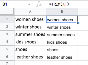
Often, after collecting data from different sources, a problem arises: the data may not be suitable for pivot tables and analysis due to extra-spaces at the beginning and end of a cell. To solve this issue, you can use the TRIM function.

Syntax:

=TRIM(text)

Example

Let’s say you have a keyword list for a website selling shoes. This list was collected from various sources. You have already deleted extra characters, but there are extra spaces too. You can remove them easily.

To do this, enter the TRIM formula in the next column and drag it down to the end of the keyword list.

Then, copy and paste only the values ​​into the original column using Paste Special.

SUBSTITUTE: Replace Letters or Symbols in Cells

Your keywords may contain the “+” modifiers, but you can quickly delete them.

Syntax:

=SUBSTITUTE (text_to_search, search_for, replace_with, [occurrence_number])

Example

Let’s see how this works and remove the “+” signs from the keywords in column A. In the B1 cell, enter the formula =SUBSTITUTE. Choose the cell you want to remove the plus signs from. Write “+” in the first quotes. Leave the second quotes empty—this means you replace the plus sign with an empty character.

Next, drag the formula down to the end of the list, select the column, copy and paste only the values ​​into the original column with Paste Special.

By default, the function changes all matches in the text. If you want to replace only one specific match, indicate its occurrence number at the end of the formula. If you don’t need it, just leave the last part out.

It’s even easier with PromoNavi’s Keyword Wrapper. Just enter your keyword list, and this tool will convert it into seven separate lists with different match types. The tool removes special symbols (+ and -) and duplicates and puts keywords to lowercase.

Start your 14-day FREE trial>>

VLOOKUP: Compare the Values of Two Data Ranges and Display Inconsistencies

The VLOOKUP (Vertical Lookup) function allows you to compare data from one column with data from another and display all inconsistencies in a separate column.

Syntax:

=VLOOKUP (search_key, range, index, [is_sorted])

Example #1

You have two keyword lists; one from Google Ads and the second one from Microsoft Ads. You need to find keywords in the Google Ads campaign (column A) that are missing on the Microsoft Ads list (column D).

In the brackets of the =VLOOKUP function, enter:

• Search key – This is a value to search for.
• Range – This is a range to consider for the search. In our example, the range is D1:D6. The function will search the first column in the range for the key specified in search_key.
• Index — The column index of the value to be returned, where the first column in the range is numbered 1.
• Is_sorted [optional]. This value indicates whether the column to be searched (the first column of the specified range) is sorted, in which case the closest match for search_key will be returned. 0 — FALSE, 1 — TRUE.

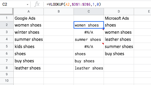
Lines marked with N/A are missing keywords: you can find them in the Google Ads campaign, but not in Microsoft Ads.

Example #2

Let’s say you need to combine two different reports. One of them contains stats on Microsoft Ads campaigns; the other contains data on Google Analytics conversions.

Copy the conversion data to the Microsoft Ads stats sheet. Add column G with conversions and enter the function =VLOOKUP in the G3 cell.

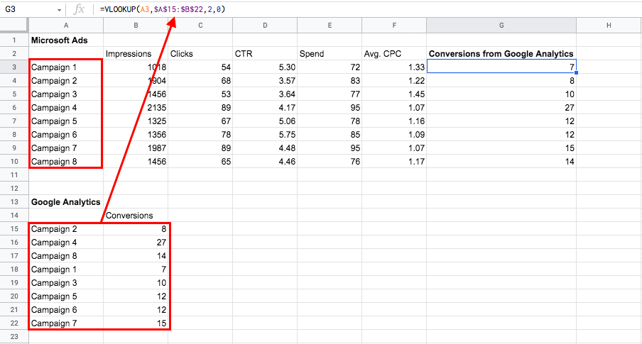
In brackets, indicate the first cell in the campaign list with statistics from Microsoft Ads — A3. Then select the data range you want to pull up conversions (this is the data from A15:B22). After the semicolon, enter the column number from the selected range (in this case, the second column). And finally, enter 0 — to indicate that you only need the exact value.

Drag the formula down to the end of the list, select the column, copy and paste only the values ​​into the original column using Paste Special.

LOWER: Сonvert Letters to Lowercase

This function converts a specified string to lowercase.

Syntax:

=LOWER(text)

Example

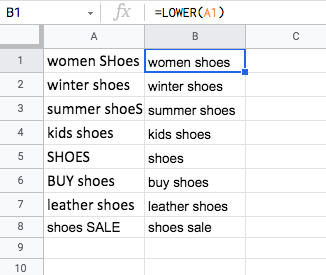
Let’s say when you were collecting keywords, you included in the list words in different cases. To bring the keyword list to a single format, use the LOWER function.

To do this, enter =LOWER in the column B cells and indicate the cell number (in our example, it is A1).

Then, drag the formula down to the end of the list, select the column, copy and paste only the values ​​into the original column using Paste Special.

Alternatively, use PromoNavi’s Keyword Wrapper. It automatically puts keywords to lowercase.

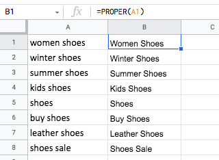
PROPER: Create Ad Headlines From Keywords

PROPER function capitalizes each word in a specified string.

Syntax:

=PROPER (text)

Example

For instance, this function will help you if you want to create ad headlines from keywords. To capitalize each word in the string, use the =PROPER function.

Drag the formula down to the end of the list, select the column, copy and paste only the values ​​into the original column using Paste Special.

LEN: Detect the Number of Characters in the Cell

Use this function to find the length of a string. This can be very helpful when writing ad headlines and texts.

Syntax:

=LEN(text)

Example

Let’s say you have headlines created from keywords, and you need to bring them in line with the character limits in Google Ads.

Let’s use the =LEN function. In brackets, specify the cell in which you want to count the characters.

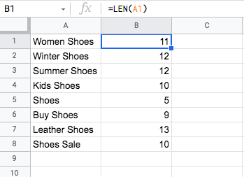
Drag the formula down to the end of the list to find inconsistencies. If the headline is too long, correct it.

IFERROR: Find Keywords to Group them

Use this function to check the formula for errors in the first argument. It returns the first argument if it is not an error value. Otherwise, it returns the second argument if present or a blank if the second argument is absent.

Syntax:

=IFERROR (value, [value_if_error])

Example

Let’s say you want to group keywords by morphology. Using the IFERROR function, you can find matching keywords from your list and specify an ad group name next to them in a new column.

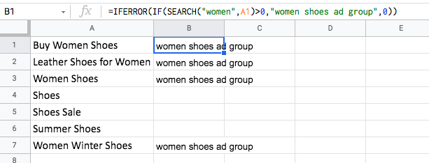
Next, drag the formula down to the end of the list, select the column, copy and paste only the values ​​into the original column using Paste Special. Now, you can filter keywords by group name.

SPLIT: Split Keywords to Separate Words and Find Negative Keywords

This function divides text around a specified character or string and puts each fragment into a separate cell in the row.

Syntax:

SPLIT (text, delimiter, [split_by_each], [remove_empty_text])

Example

If you need to find negative keywords in your keyword list, you can do it quickly by using the SPLIT function. 

Enter the =SPLIT function in the column right to the column with the keywords you want to split:

• Specify the cell number you want to divide.
• Next, enter the character or characters to use to split text.

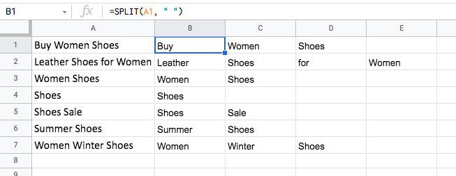
Drag the formula down. As you can see, each word has its own cell. Now, you can remove duplicates, alphabetize them and leave only negative keywords.

Alternatively, try PromoNavi’s Add Negative Keyword tool. It analyzes your PPC performance and shows queries with poor performance. You can add negative keywords to your Google Ads campaigns directly from PromoNavi in one-click.

Start your 14-day FREE trial>>

CONCATENATE: Combine Text in Cells and Generate UTM Tags

With this function, you can combine multiple text elements in one line.

Syntax:

=CONCATENATE(string1, [string2, …])

Example

Let’s say for each keyword, you need to create a link with a UTM-tag. 

Let’s use the =CONCATENATE function and create for each keyword a link with UTM-tag where utm_term will be the keyword.

The first column should contain the keywords; the second one — the landing pages; the third one — UTM-tags ending with utm_term=. In the Final URL column, use the =CONCATENATE function. Select the cells in the order you want to combine them. In this example, it would be URL (B2), UTM (C2), and keyword (A2).

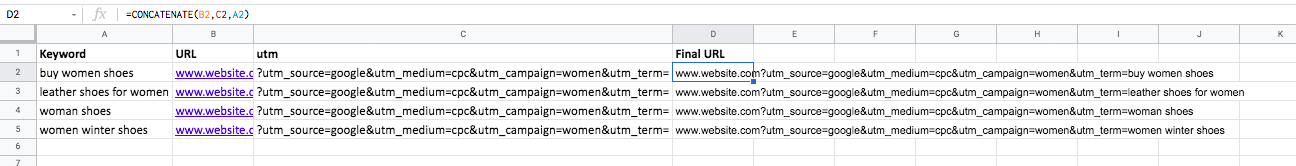
After that, drag the formula down to the end of the list, select the column, copy and paste only the values ​​into the original column using Paste Special so that you don’t lose the data.

REGEXEXTRACT: Extract Text from the Cells

This function extracts matching substrings according to a regular expression.

Syntax:

=REGEXEXTRACT(text, regular_expression)

Example

Let’s say you want to collect competitor domains to target “Custom Audiences” in Google Ads. You don’t need the exact landing page, but only the domain name. 

To quickly extract the domain name, let’s apply the REGEXEXTRACT formula with the following regular expression:

^(?:https?:\/\/)?(?:[^@\n]+@)?(?:www\.)?([^:\/\n]+)

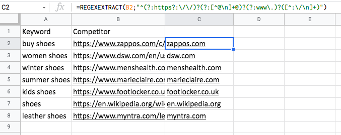
Drag the formula down to the end of the list. Alphabetize your domains and delete irrelevant URLs. Now you can upload your list to «Custom Audiences» in Google Ads. 

GOOGLETRANSLATE: Translate Keywords and Other Text

This function translates text from one language into another.

Syntax:

=GOOGLETRANSLATE(text, [source_language], [target_language])

Example

Let’s say you want to launch a campaign in Germany, and you need to translate keywords quickly. Let’s use the =GOOGLETRANSLATE function.

To do this, insert the formula into the next column:

=GOOGLETRANSLATE(A1;”en”;”de”)

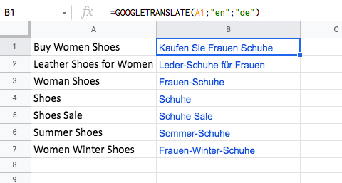
Select the keyword list you have translated, again copy and paste only the values.

With this feature, you can translate into any language ​​supported by Google.

IMPORTRANGE: Import Data from Other Sheets

The function imports a range of cells from one spreadsheet to another.

Syntax:

=IMPORTRANGE(spreadsheet_url, range_string)

Example

Let’s create a report for Google Ads and Facebook Ads taking data from two spreadsheets. To combine this data on a single sheet, use the IMPORTRANGE function.

To do this, enter a link to the table in the function. After the semicolon, specify the sheet and the data range.

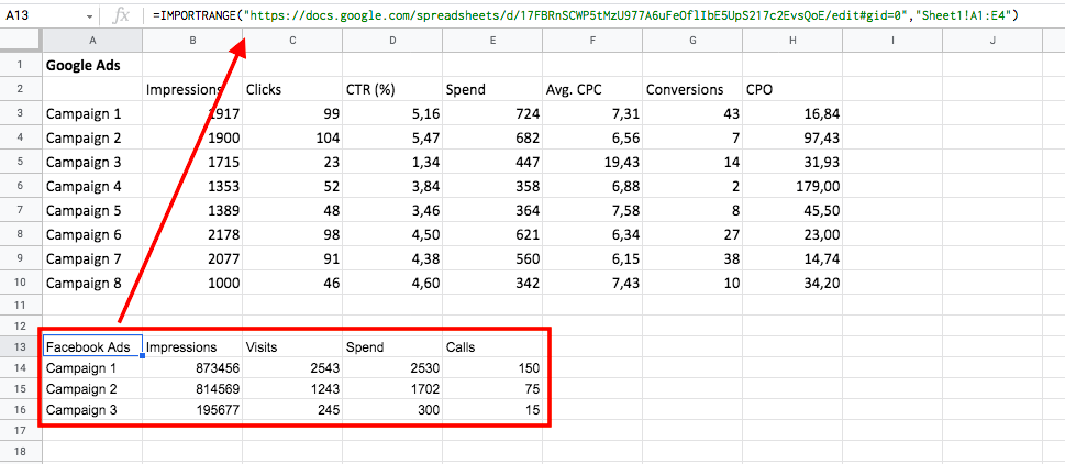
The data will be loaded and displayed in this report. The only thing to keep in mind is that you must have open access to the sheet from which you are uploading data.

In that way, you can display the data you want to give access to clients or other professionals, but they won’t get access to the original reports.

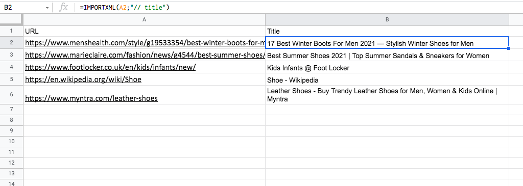
IMPORTXML: Check Title and H1 Content on Landing Pages

IMPORTXML imports data from any structured data type online.

When you launch Dynamic Ads on Google Ads, you need to make sure that the landing pages contain relevant Title and H1 tags. You can use the IMPORTXML function to check them.

Syntax:

=IMPORTXML(url, xpath_query)

Example

Let’s say you need to check if the title tags on the landing pages are filled out. In the first column, enter the URLs of the pages you want to check, and in the next column, the =IMPORTXML formula. The XPath-request for Title parsing is “// title.”

Using the IMPORTXML function, you can get almost any data from a page. Here are examples of other XPath queries:

• Get all H1 tags (or H2-H6): //h1
• Get the meta description: //meta[@name=’description’]/@content
• Get meta keywords: //meta[@name=’keywords’]/@content
• Extract email addresses: //a[contains(href, ‘mailTo:’) or contains(href, ‘mailto:’)]/@href
• Get links to social media profiles: //a[contains(href, ‘twitter.com/’) or contains(href, ‘facebook.com/’) or contains(href, ‘instagram.com/’) or contains(href, ‘youtube.com/’)]/@href

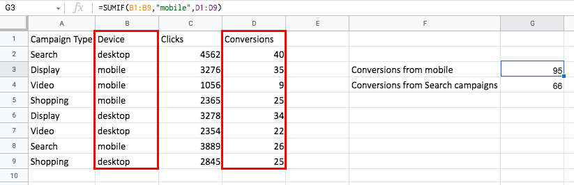
SUMIF: Find the Sum of Cells Content That Meet a Certain Condition

This function finds the sum of the contents of the cells that match a certain condition.

Syntax:

=SUMIF(range, criterion, [sum_range])

Example

You have downloaded a report from Google Analytics with a breakdown by campaign and device type. You need to calculate how many registrations you get from mobile users and Search campaigns.

To do this, use the SUMIF function. Enter in brackets the range you want to test against criterion; after the semicolon, indicate the condition (in our example, it is “Search”); then enter the range you want to summarize.

That’s how you can calculate the registration number or clicks for each item:

TRANSPOSE: Swap Rows and Columns

The function swaps the positions of the rows and columns in an array of cells.

Syntax:

=TRANSPOSE(array_or_range)

Example

You have data in a pivot table from the previous example. But it is not convenient to analyze and compare the campaign types with each other when they stand in rows. To display the same data in columns, use the TRANSPOSE function.

In an empty cell, enter = TRANSPOSE and specify the range — in this example, this is A1: E5.

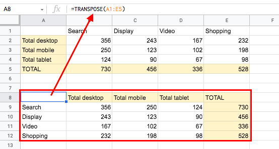
Campaign types are now in columns without losing data.

Try out these helpful functions and share this article with other PPC professionals!

If you need more in-depth PPC automation, try PromoNavi platform to solve everyday tasks and reach your marketing KPIs faster. With PromoNavi, you can:

• Automate PPC reporting, competitor analysis, keyword research
• Track your PPC performance across accounts on a single dashboard
• Get optimization suggestions, and many more